By the tiswa editorial team, from the official sources listed at the end of this guide. How we write our guides
This Google Sheets guide covers the free, browser-based alternative to Excel, and the one thing it does better for students: several people working in the same file at the same time. A Google Account is all you need. We start from scratch: creating a sheet, sharing it with the right permissions, freezing headers, sorting and filtering, conditional formatting, then linking a Google Form to collect survey or project data.
Create your first sheet
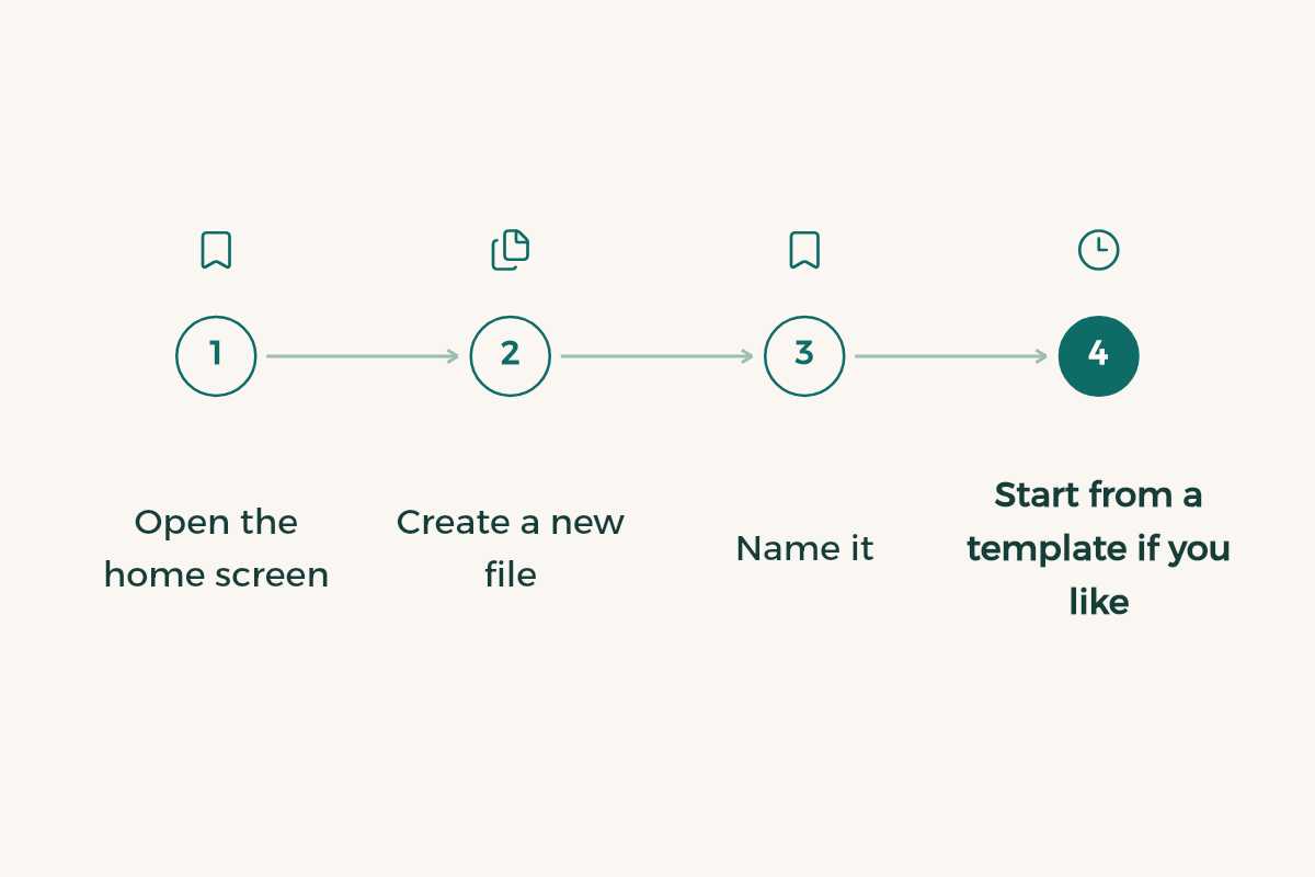
- Open the home screen
Go to sheets.google.com and sign in with your Google Account.
- Create a new file
Click New (the plus icon) and a new spreadsheet opens. Google's help also notes you can go to sheets.google.com/create to start straight away.
- Name it
Click "Untitled spreadsheet" at the top and give it a clear name with the course and topic, so it is easy to find in Drive.
- Start from a template if you like
Google offers ready templates, which may already fit a budget, a weekly schedule or a task tracker.
Share with the right permission
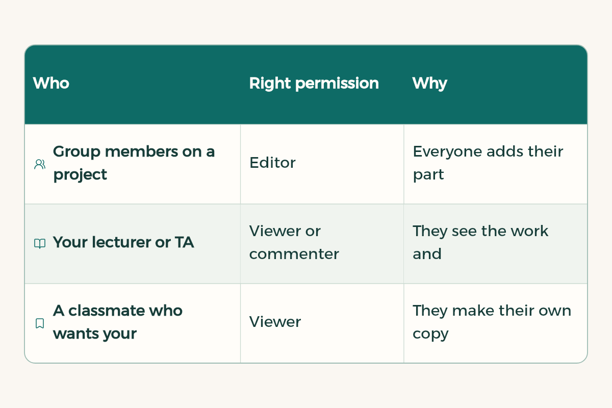
According to Google's help, when you share a file you choose for each person whether they can view, comment or edit. That choice matters more than it looks:
| Who | Right permission | Why |
|---|---|---|
| Group members on a project | Editor | Everyone adds their part directly |
| Your lecturer or TA | Viewer or commenter | They see the work and comment without changing data by accident |
| A classmate who wants your template | Viewer | They make their own copy and leave yours alone |
Google Sheets also supports comments, action items and emoji reactions. On group projects, comment on a cell and mention your teammate instead of messaging on the side, so the discussion stays next to the cell it is about.
Freeze the header row
In a long sheet, the headers scroll out of view and you lose track of which column you are reading. Google explains that freezing keeps rows or columns visible while you scroll:
- Select the row
Pick the row or cell you want to freeze up to.
- Open the menu
At the top, click View, then Freeze.
- Choose how many
Select how many rows or columns to freeze. One header row is usually enough.
Google recommends freezing the first row before sorting when it holds headers, so they do not get mixed into the data.
Sort and filter
A filter temporarily hides rows you do not need, so you can focus on one college's responses or one spending category without deleting anything.
- Select the range
Select your data including the header row.
- Create the filter
Go to Data, Create a filter. A filter icon appears at the top of each column.
- Pick how to filter
Click the icon and filter by condition, by values (untick the ones to hide), or by colour.
Google notes that filtering by colour works with conditional formatting colours but not with alternating colours. If Create a filter is unavailable, the usual cause is merged cells or hidden rows and columns: unmerge and unhide, then try again.
Conditional formatting: colour data automatically
Conditional formatting changes a cell's colour based on its value, so low marks or close deadlines stand out without searching. Google's method: select the cells, then Format, Conditional formatting, and set a rule.
- A ready rule: such as "Less than" 60 in red for a marks column.
- A text rule: such as "Text contains" "Not submitted" in a status column.
- A custom formula rule when the condition depends on more than one cell.
One of Google's own examples highlights duplicates with the custom formula =COUNTIF($A$1:$A$100,A1)>1. That is handy for spotting a repeated student ID in an attendance list, or a duplicate survey response before analysis.
Collect research data with a linked form
From inside Google Sheets you can create a Google Form linked straight to the file. Per Google's help: open the spreadsheet, then Tools, Create a new form. A new sheet is added for responses and the form opens so you can write your questions. Each new response lands as a row on that sheet automatically, ready for filters, formatting and formulas.
How to write questions, pick question types and set up the form is covered in the Google Forms guide.
Formulas in Google Sheets
Most core functions work under the same names in Google Sheets: SUM, AVERAGE, IF, COUNTIF, SUMIF and VLOOKUP. What you learn in basic Excel formulas and VLOOKUP and XLOOKUP carries over. Absolute references with $ work the same way, as in the duplicates example above.
Worked example: a group project tracker
- Create the file
A new sheet named after the course and project, with columns: task, owner, due date, status, link.
- Freeze the headers
View, Freeze, one row.
- Share it
Add teammates as editors, and your lecturer as a commenter if they want to follow progress.
- Colour the status
Conditional formatting: "Done" in green and "Late" in red.
- Filter your tasks
Each member filters the owner column to see only their own tasks.
- Discuss in comments
Any question about a task goes in a comment on its cell, mentioning the owner.
Habits that keep a shared file tidy
- Keep one sheet for raw data that people only add to, and a second sheet for calculations and summaries, so nobody wipes a formula by accident.
- Write two lines on the first sheet explaining what the file holds and who owns each part, so any new group member understands it.
- Standardise data entry: the same status wording and the same date format, because filters and conditional functions rely on exact matches.
- Do not merge cells inside the data area; as Google notes, merging gets in the way of filtering and sorting.
- Before a big change, make a copy of the file and try it there, then bring the result back to the original.
- Give sheets clear names instead of Sheet1 and Sheet2, such as Responses, Analysis and Tasks.
Google Sheets or Excel?
| Situation | Better fit |
|---|---|
| A group project where everyone edits at once | Google Sheets |
| Collecting survey responses | Google Sheets with Google Forms |
| A course that asks for an Excel file or advanced PivotTable features | Excel, usually free with your university email |
| A slow or shared computer | Google Sheets in the browser |
To get Excel free, read Office for students, and to make more of your university account, read university email benefits.
I have a Google Sheets table: column A is [describe it], column B is [describe it], and the data runs from row 2 to [number]. I want to colour the whole row when [condition]. Write the custom formula for conditional formatting, tell me which range to select before entering it, and explain why the $ signs go where they do.
- Google AI: Google AI offers Google AI Plus free for a year to university students in Saudi Arabia.
- Notion: Notion offers Notion Education plan for students to university students in Saudi Arabia for free.
- WPS Office: WPS Office offers WPS Office for free to university students in Saudi Arabia.