By the tiswa editorial team, from the official sources listed at the end of this guide. How we write our guides
Charts in Excel can turn a full page of numbers into one figure in a lab report, research paper or presentation. Pick the wrong type, though, and the chart confuses rather than clarifies. This guide follows Microsoft's method for creating a chart in seconds, then helps you choose the right type for each kind of student data, add titles and a trendline, and prepare the final figure for a paper or slides.
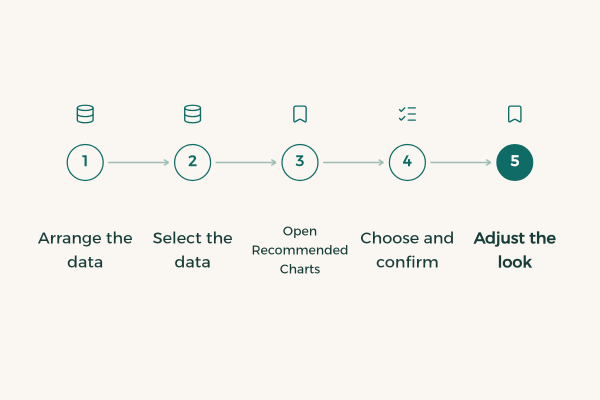
Create a chart in under a minute
- Arrange the data
Put categories in one column (course names or months, say) and values in the next, with a header row on top.
- Select the data
Select the headers and the values together.
- Open Recommended Charts
Go to Insert, Recommended Charts. Excel shows suggested types for your data with a preview of each.
- Choose and confirm
Pick the one closest to what you want to say, then OK.
- Adjust the look
On the Chart Design tab, try the quick layouts and chart styles, which are ready sets of matching colours and effects.
Which type fits your data?
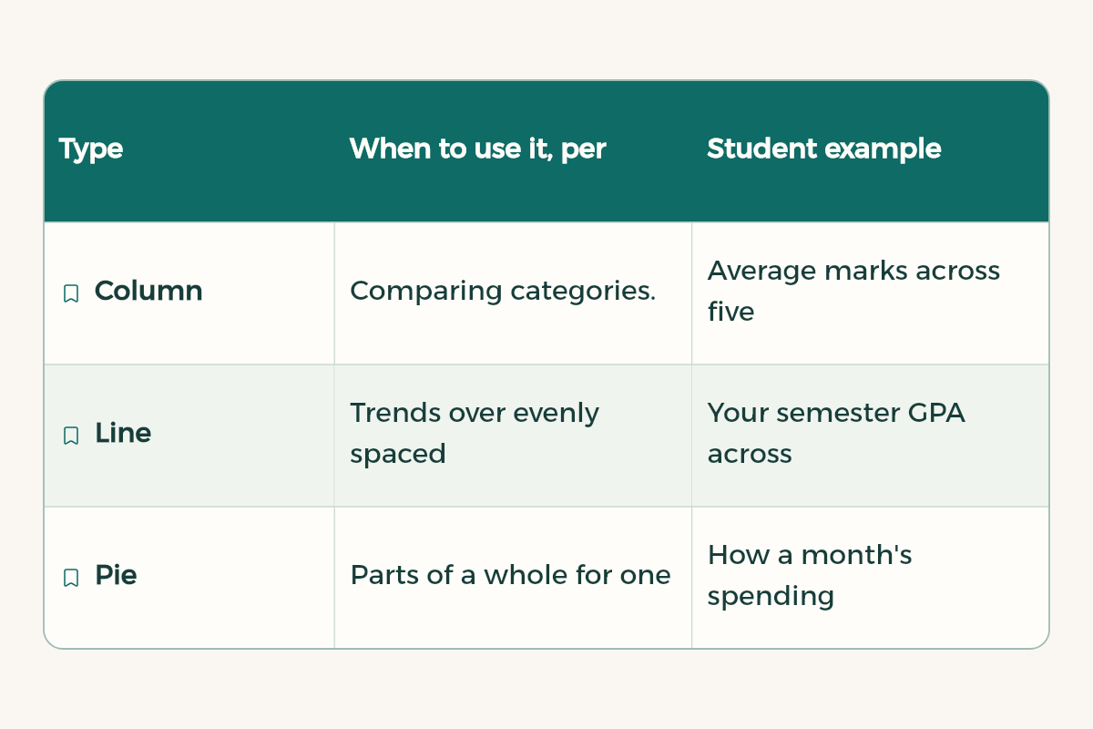
These are the main chart types as Microsoft describes them, with university examples:
| Type | When to use it, per Microsoft | Student example |
|---|---|---|
| Column | Comparing categories. Stacked shows totals; 100% stacked shows each part's contribution to the whole | Average marks across five courses |
| Line | Trends over evenly spaced intervals such as months or quarters; works well with several series | Your semester GPA across years |
| Pie | Parts of a whole for one series, no negative values, no more than about seven categories | How a month's spending splits by category |
| Doughnut | Parts of a whole with several series, but harder to read than stacked columns | Rarely needed; prefer stacked columns |
| Bar | Comparing individual items, especially with long labels | College names in survey results |
| Area | Change over time and the contribution of parts to a total | Study hours per course across weeks |
| Scatter | The relationship between two numeric values; for scientific, statistical and engineering data | Concentration vs absorbance in a lab |
| Radar | Comparing aggregate values of several series around a centre point | Rating skills in a group project |
A quick rule: if your question is "which is bigger?", use column or bar. If it is "how did it change?", use line. If it is "what share is each part?" and you have few categories, use pie; otherwise 100% stacked columns. If it is "are these two variables related?", use scatter.
Chart elements: what should show
Microsoft lists the common chart elements as the chart title, axis titles and labels, the legend, gridlines, tick marks and the plot area. You can show, hide, move or reformat any of them.
- The title should state the finding, not the data name. "Satisfaction peaks in fourth year" says more than "Average satisfaction".
- Axis titles are essential in lab work: always include the unit, such as time (s) or concentration (mol/L).
- Remove the legend when there is only one series; it adds nothing.
- Lighten or remove gridlines if they pull attention away from the data.
Trendlines for lab results
If you have readings from an experiment and want to show the overall relationship, add a trendline.
- Draw a scatter chart
Select the two value columns, then Insert and choose a Scatter chart.
- Add the line
Select the chart, then Chart Design, Add Chart Element, Trendline.
- Pick the type
Microsoft's options are Linear, Exponential, Linear Forecast and Moving Average.
- Explain it
Under the figure in your report, write a sentence on what the line means. Do not leave the picture to speak alone.
Choose the trendline type based on what the theory behind your experiment predicts, not on which looks best. If you are unsure, ask your lab instructor or check the lab manual.
Worked example: your monthly budget chart
- Summarise spending
Use SUMIF per category as in basic Excel formulas, or a PivotTable as in pivot tables in Excel.
- Cut the categories
If you have more than about seven categories, group the small ones into "Other" so a pie chart stays readable.
- Draw it
Select the category totals, then Insert, Recommended Charts, and choose Pie or Column.
- Compare months
With more than one month, use clustered columns: each category a group, each month a colour.
Third example: one survey question
Agree-disagree survey questions read better as bars than as a pie, because the options are ordered and their labels are fairly long.
- Count the answers
For each option from "Strongly agree" to "Strongly disagree", count responses with COUNTIF or a PivotTable.
- Keep the order
List options in the same order as the survey, not largest to smallest, so readers follow the scale.
- Draw bars
Insert, Recommended Charts, and choose Bar. Long labels show in full on the axis.
- Show shares
With many responses, chart percentages instead of counts and give the sample size in or under the title.
Common chart mistakes
| Mistake | Why it hurts | Instead |
|---|---|---|
| A pie with ten or more slices | Small slices cannot be read | Columns or bars, or group small ones as "Other" |
| A column chart axis that does not start at zero | It exaggerates small differences | Start column chart axes at zero |
| Lines for data that is not over time | It suggests a trend that is not there | Columns for separate categories |
| Many colours with no meaning | They distract the reader | One colour, with the key result highlighted |
| No title or units | It cannot be understood out of context | A title stating the finding, axes with units |
Prepare the chart for a paper or slides
- Enlarge label and number fonts, because what looks clear on your screen shrinks a lot on slides and printed pages.
- Use one strong colour for the key result and muted colours for the rest.
- Number figures in your paper (Figure 1, Figure 2) and give the data source under each.
- When you paste into PowerPoint or Word, make sure resizing does not distort the proportions.
- Avoid 3D effects; they make values harder to compare.
Full presentation advice is in how to make a presentation, and writing the results around your figures is in how to write a research paper.
Ask AI to pick the chart
I have data in Excel: [describe the columns and number of rows]. I want to show the reader that [the point you want to make]. Which chart type fits best and why? Suggest a chart title and axis titles, and tell me whether to add a trendline.
If you work in the browser, charts are also available in Google Sheets. The full starter guide is Excel for students.
- WPS Office: WPS Office offers WPS Office for free to university students in Saudi Arabia.
- Notion: Notion offers Notion Education plan for students to university students in Saudi Arabia for free.
- Google AI: Google AI offers Google AI Plus free for a year to university students in Saudi Arabia.