By the tiswa editorial team, from the official sources listed at the end of this guide. How we write our guides
Excel for students is not just for accounting majors. You will use it to work out your expected grade, plan a monthly budget, analyse your graduation project survey and chart lab results. The good news: about ten formulas cover most of what a student needs. This guide gives you each one with an example you can copy.
Get Excel free
Microsoft gives Office 365 A1 free to students with an eligible education email, including Excel for the web alongside Word and PowerPoint. The full details, the difference between A1 and A3, and what happens after graduation are in Office for students.
Core formulas with student examples
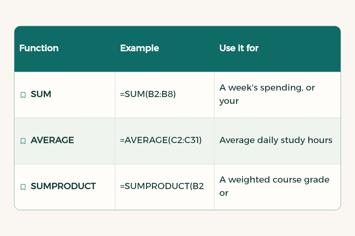
| Function | Example | Use it for |
|---|---|---|
| SUM | =SUM(B2:B8) | A week's spending, or your coursework marks |
| AVERAGE | =AVERAGE(C2:C31) | Average daily study hours over a month |
| SUMPRODUCT | =SUMPRODUCT(B2:B6,C2:C6)/SUM(C2:C6) | A weighted course grade or a GPA: mark times weight or hours, divided by the total |
| IF | =IF(D2>=60,"Pass","Review") | Labelling a mark against a threshold your course sets |
| COUNTIF | =COUNTIF(E2:E40,"Submitted") | How many assignments you have handed in |
| ROUND | =ROUND(F2,2) | Rounding your GPA to two decimal places |
| MAX and MIN | =MAX(C2:C31) | Highest and lowest values in lab results |
| XLOOKUP | =XLOOKUP(H2,A2:A50,C2:C50,"Not found") | Finding a student by ID and returning their mark |
Worked example: your expected course grade
- List the components
In column A, list the grade components from your syllabus: assignments, midterm 1, midterm 2, project, final.
- Add the weights
In column B, each component's weight out of 100. Check that =SUM(B2:B6) equals 100.
- Add your marks
In column C, your mark out of 100 for each finished component. Leave the final empty.
- What you have so far
In a new cell: =SUMPRODUCT(B2:B5,C2:C5)/100 gives the points you have already earned out of the total.
- What you need in the final
If your target is 85 out of 100 and the final's weight is in B6: =(85-E2)/B6*100, where E2 holds what you have so far. The result is the mark you need in the final, out of 100.

The same idea gives you your semester GPA: put each course's grade points in one column and its credit hours in another, use SUMPRODUCT, then divide by total hours. Grade point scales differ between universities, so check your university's regulations.
Example three: tracking attendance
Some courses bar students whose absences pass a limit set by their university's rules. Build a simple sheet to track yourself:
- Column A
The date of each lecture.
- Column B
Write "present" or "absent".
- Count cell
Type =COUNTIF(B2:B40,"absent") to count absences.
- Percentage cell
Divide absences by the total number of lectures and format the cell as a percentage.
- Visual warning
Use conditional formatting to colour the percentage cell red as it nears your university's limit.
You know where you stand at any moment instead of being surprised at the end of term.
Common mistakes that give wrong results
- Copying a formula down without locking references. To keep a cell fixed, such as the weight cell, write it with dollar signs like $C$1.
- Numbers stored as text, often shown with different alignment. Convert them before summing.
- Extra spaces in names that stop a lookup finding the value. Clean them before using XLOOKUP.
- Merged cells inside a data table. Merging breaks sorting and pivot tables, so keep it for headings only.
A routine that makes you fast in Excel
- Spend fifteen minutes a week applying one new function to your own data, such as spending or grades.
- Keep one practice file to return to when you forget a formula.
- Learn the core keyboard shortcuts in keyboard shortcuts for students.
Second example: a monthly budget
- Income
At the top, list your monthly income: stipend, family allowance or part-time work, and total it with SUM.
- Spending by category
A table with columns: date, category (food, transport, subscriptions, study, fun), amount. Turn it into an Excel table so it grows as you add rows.
- Total per category
Use SUMIF, such as =SUMIF(B2:B100,"Food",C2:C100), to see what you spent on food.
- What is left
Subtract total spending from income, and use conditional formatting to colour the cell when it drops below an amount you choose.
- A chart
Select the category totals and insert a pie chart to see where most of your money goes.
If subscriptions or eating out are among your biggest categories, that is where student discounts help most. If you receive a monthly stipend, see student stipend dates.
XLOOKUP for big tables
According to Microsoft's support page, XLOOKUP searches one column for a value and returns the result from the same row in another column, whichever side the return column is on. The syntax:
=XLOOKUP(lookup_value, lookup_array, return_array, [if_not_found], [match_mode], [search_mode])
- The first three arguments are required: what you look for, where you look, and where the answer comes from.
- if_not_found is optional: the text to show when there is no match. Without it you get #N/A.
- The default match is exact, so most of the time you add nothing else.
- XLOOKUP is not available in Excel 2016 or Excel 2019. If your college lab runs those versions, use Excel for the web.
PivotTables for survey analysis
If you ran a survey for a project or paper, a PivotTable summarises hundreds of responses in seconds. Microsoft's steps for Excel for Windows:
- Shape the data
One question per column, a single header row at the top, and one response per row.
- Insert the PivotTable
Select the data, then Insert, PivotTable.
- Choose where
New Worksheet, then OK.
- Add fields
Tick fields in the PivotTable Fields pane. Non-numeric fields go to Rows, dates and times to Columns, and numbers to Values by default. Drag any field to move it.
- Refresh after adding
When you add new responses to the source data, refresh the PivotTable to include them.
Then use conditional formatting to colour cells by value, such as marks below a threshold in red, so patterns jump out. Microsoft notes it works on a cell range or an Excel table, and in Excel for Windows on a PivotTable too.
Let AI write the formula
I have an Excel sheet: column A has course names, B credit hours, C the mark out of 100, D grade points. Write a formula that calculates [what you want], explain each part on its own line, and tell me which cell to put it in.
To organise tasks rather than numbers, try Notion for students. To present your results, read how to make a presentation. And survey results need clear write-up, see how to write a research paper.
- WPS Office: WPS Office offers WPS Office for free to university students in Saudi Arabia.
- Notion: Notion offers Notion Education plan for students to university students in Saudi Arabia for free.
- Google AI: Google AI offers Google AI Plus free for a year to university students in Saudi Arabia.